
Causation has long been something of a mystery, bedeviling philosophers and scientists down through the ages. What exactly is it? How can it be measured — that is, can we assess the strength of the relationship between a cause and its effect? What does an observed association between factors — a correlation — tell us about a possible causal relationship? How do multiple factors or causes jointly influence outcomes? And does causation even exist “in the world,” as it were, or is it merely a habit of our minds, a connection we draw between two events we have observed in succession many times, as Hume famously argued? The rich philosophical literature on causation is a testament to the struggle of thinkers throughout history to develop satisfactory answers to these questions. Likewise, scientists have long wrestled with problems of causation in the face of numerous practical and theoretical impediments.
Yet when speaking of causation, we usually take for granted some notion of what it is and how we are able to assess it. We do this whenever we consider the consequences of our actions or those of others, the effects of government interventions, the impacts of new technologies, the consequences of global warming, the effectiveness of medical treatments, the harms of street drugs, or the influence of popular movies. Some causal statements sound strong, such as when we say that a treatment cured someone or that an announcement by the government caused a riot. Others give a weaker impression, such as when we say that the detention of an opposition leader affected international perceptions. Finally, some statements only hint at causation, such as when we say that the chemical bisphenol A has been linked to diabetes.
In recent years, it has become widely accepted in a host of diverse fields, such as business management, economics, education, and medicine, that decisions should be “evidence-based” — that knowledge of outcomes, gathered from scientific studies and other empirical sources, should inform our choices, and we expect that these choices will cause the desired results. We invest large sums in studies, hoping to find causal links between events. Consequently, statistics have become increasingly important, as they give insight into the relationships between factors in a given analysis. However, the industry of science journalism tends to distort what studies and statistics show us, often exaggerating causal links and overlooking important nuances.
Causation is rarely as simple as we tend to assume and, perhaps for this reason, its complexities are often glossed over or even ignored. This is no trifling matter. Misunderstanding causal links can result in ineffective actions being chosen, harmful practices perpetuated, and beneficial alternatives overlooked. Unfortunately, the recent hype about “big data” has encouraged fanciful notions that such problems can be erased thanks to colossal computing power and enormous databases. The presumption is that sheer volume of information, with the help of data-analysis tools, will reveal correlations so strong that questions about causation need no longer concern us. If two events occur together often enough, so the thinking goes, we may assume they are in fact causally linked, even if we don’t know how or why.
As we will see, understanding causation as best we can remains indispensable for interpreting data, whether big or small. In this essay we will mostly leave aside the rich and complex philosophical literature on causation, instead focusing our attention on more practical matters: how we should think about causation and correlation in medicine, politics, and our everyday lives. We will also discuss some remarkable advances in thinking about cause-and-effect relationships, advances made possible by a confluence of ideas from diverse branches of science, statistics, and mathematics. Although in-depth understanding of these developments requires specialized technical knowledge, the fundamental ideas are fairly accessible, and they provide insight into a wide range of questions while also showing some of the limitations that remain.
Let us begin with a familiar example. We know that smoking causes lung cancer. But not everyone who smokes will develop it; smoking is not a sufficient cause of lung cancer. Nor is smoking a necessary cause; people who do not smoke can still develop lung cancer. The verb “to cause” often brings to mind unrealistic notions of sufficient causation. But it is rare that an event has just one cause, as John Stuart Mill noted in A System of Logic (1843):
It is seldom, if ever, between a consequent and a single antecedent that this invariable sequence subsists. It is usually between a consequent and the sum of several antecedents; the concurrence of all of them being requisite to produce, that is, to be certain of being followed by, the consequent.
Based on similar insights in a number of fields, including philosophy, law, and epidemiology, scholars have in recent years proposed models of jointly sufficient causation to show how multiple causes can be responsible for one outcome. It has become common with the help of such models to express causation in terms of probability: when just one factor, such as smoking, is known to have a probable influence on an effect, any impression of sufficient causation can be avoided by simply saying that smoking “promotes” lung cancer. Probability modeling can be seen as a strategy for simplifying complex situations, just as models in mechanics involve simplifications like objects falling in a vacuum or sliding down a frictionless plane.
The occurrence of lung cancer may depend on numerous factors besides smoking, such as occupational exposure to hazardous chemicals, genetic predisposition, and age. Some factors may be entirely unknown, and others poorly understood. In many cases, measurements of some factors may not be available. Thinking of causation in terms of probability allows us to simplify the problem by setting aside some of these factors, at least tentatively.
Ironically, a leading opponent of the claim that smoking causes lung cancer was geneticist Ronald A. Fisher, one of the foremost pioneers of modern statistical theory. A number of studies showed an association between smoking and lung cancer, but Fisher questioned whether there was enough evidence to suggest causation. (Although technical distinctions between correlation and association are sometimes made, these terms will be used synonymously in this essay.) Fisher pointed out, for instance, that there was a correlation between apple imports and the divorce rate, which was surely not causal. Fisher thereby launched a cottage industry of pointing out spurious correlations.
The fact that Fisher was himself a smoker and a consultant to tobacco firms has at times been used to suggest a conflict of interest. But even if he was wildly off base regarding the link between smoking and lung cancer, his general concern was valid. The point is often summed up in the maxim, “Correlation is not causation.” Just because two factors are correlated does not necessarily mean that one causes the other. Still, as Randall Munroe, author of the webcomic xkcd, put it: “Correlation doesn’t imply causation, but it does waggle its eyebrows suggestively and gesture furtively while mouthing ‘look over there.’” We are tempted to think of correlation and causation as somehow related, and sometimes they are — but when and how?
The modern debate over correlation and causation goes back to at least the mid-eighteenth century, when Hume argued that we can never directly observe causation, only “the constant conjunction of two objects.” It is perhaps not surprising that scientists and philosophers have had mixed feelings about causation: on the one hand it appears to be central to the scientific enterprise, but on the other hand it seems disconcertingly intangible. To this day, debate continues about whether causation is a feature of the physical world or simply a convenient way to think about relationships between events. During the eighteenth and nineteenth centuries, statistical theory and methods enjoyed tremendous growth but for the most part turned a blind eye to causation. In 1911, Karl Pearson, inventor of the correlation coefficient, dismissed causation as “another fetish amidst the inscrutable arcana of even modern science.” But developments in the 1920s began to disentangle correlation and causation, and paved the way for the modern methods for inferring causes from observed effects. Before turning to these sophisticated techniques, it is useful to explore some of the problems surrounding correlation and causation and ways of resolving them.
A source of confusion about causation is that news reports about research findings often suggest causation when they should not. A causal claim may be easier to understand — compare “seat belts save lives” with “the use of seat belts is associated with lower mortality” — because it presents a cause (seat belts) acting directly (saving lives). It seems to tell a more compelling story than a correlational claim, which can come across as clumsy and indirect. But while a story that purports to explain a correlation might seem persuasive, a causal claim may not be justified. Consider the oft-cited research of the psychologist John Gottman and his colleagues about predicting divorce based on observations of couples in a conversation about their relationship and in a conflict situation. In a series of studies beginning in the 1990s, Gottman was able to predict, with accuracy as high as 94 percent, which couples would divorce within three years. Among the strongest predictors of divorce were contempt, criticism, stonewalling, and defensiveness. These are impressive findings, and have been widely reported in the media. Unfortunately, they have also been widely misinterpreted. Some newspaper and magazine articles have suggested to readers that these findings mean they can reduce their risk of divorce (or even “divorce-proof” their marriages, as some put it) by changing how they communicate, and in particular by reducing the problem behaviors that were identified. Such changes may well be helpful, but Gottman’s research does not substantiate this claim. His predictions were based on a correlation between observable behaviors and subsequent outcome. The correlation does not imply that the outcome must have been due to those behaviors. Nor does it imply that changing those behaviors would have changed the outcome. It is possible, for example, that defensiveness is a symptom of other problems in a marriage, and that reducing defensiveness would have limited benefit unless the underlying causes of the discord were addressed.
How can factors be correlated but not causally related? One reason is pure chance: Fisher’s association between apple imports and the divorce rate was just a coincidence. Today it is easy to generate such spurious correlations. With the emergence of big data — enormous data sets collected automatically, combed for patterns by powerful computing systems — correlations can be mass-produced. The trouble is that many of them will be meaningless. This is known as the problem of “false discovery.” A small number of meaningful associations is easily drowned in a sea of chance findings. Statisticians have developed theories and tools to deal with the problem of chance findings. Perhaps best known is the p-value, which can be used to assess whether an observed association is consistent with chance, or conversely, as it is commonly put, that it is “statistically significant.” At times, the idea of statistical significance becomes the source of misconceptions, including the belief that correlation does not imply causation unless the correlation is statistically significant. The flaw in this belief is easily seen in the context of large data sets, where an observed association is virtually guaranteed to be statistically significant. Sheer volume of data does not warrant a claim about causation.
Another reason why two factors may be correlated even though there is no cause-and-effect relationship is that they have a common cause. Examples of such “confounding,” as it is known, are all too common in the scientific literature. For example, a 1999 study published in Nature showed that children under the age of two who slept with night lights were more likely to have myopia. Other researchers later showed that myopic parents were more likely to keep their lights on at night. It may be that the parents were a common cause of both the use of night lights and, by virtue of genetic inheritance, the myopia passed on to their children.
In medical research, confounding can make effective treatments appear to be harmful. Suppose we review hospital records and compare the outcomes of patients with a certain disease who did and did not receive a new drug. This might sound like a good way to determine how well the drug works. However, it can easily result in what is called “confounding by indication”: certain biases may have influenced which patients received the new drug. For example, if the patients who got the new drug were the sicker ones, then even if the drug helps, the outcomes of the patients who received it may be worse than the outcomes of those who did not.
Confounding can also make ineffective treatments appear to be helpful. Suppose a patient suffers from a chronic disease whose severity waxes and wanes. When his symptoms are particularly bad he visits a quack healer and his symptoms usually improve within a week or two. The trouble is, the improvement is simply a result of the natural fluctuation of the illness. The flare-up of symptoms prompts the patient to visit the quack, but due to the natural course of illness, the flare-up is followed by improvement within a week or two. Confounding makes the visits to the quack healer appear effective.
Misleading correlations may also arise due to the way subjects are selected to be part of a study. For example, there is evidence that certain studies of an association between breast implants and connective tissue disease may have suffered from selection bias. Suppose participation in a study was greater for women with implants and also for women with connective tissue disease (perhaps these two groups were more likely to respond to a questionnaire than women from neither group). The study would then include a disproportionately large number of women with both implants and connective tissue disease, leading to an association even if there were no causation at all. Whenever the selection of subjects into a study is a common effect of both the exposure variable and the outcome, there is a risk of selection bias. It has been suggested that bias due to a common effect (selection bias) may be more difficult to understand than bias due to a common cause (confounding). This makes selection bias particularly problematic.
In the analysis of big data, selection bias may be especially pernicious because the processes that affect which individuals are included in or excluded from a database are not always apparent. Additionally, such databases are often spotty: for a variety of reasons, many records may be missing some data elements. In some cases, records that have missing values are automatically omitted from analyses, leading to another form of selection bias. In these cases, the associations detected may be nothing more than artifacts of the data collection and analysis.
So the presence of a correlation does not always mean there is a causal relationship. Perhaps more surprisingly, the reverse is true as well: the presence of a causal relationship does not always mean there is a correlation. An example of this has been attributed to the economist Milton Friedman. Suppose a thermostat keeps your home at a constant temperature by controlling an oil furnace. Depending on the outside temperature, more or less oil will be burned. But since the thermostat keeps the inside temperature constant, the inside temperature will have no correlation with the amount of oil burned. The oil is what keeps the house warm — a causal relation — but it is uncorrelated with the temperature in the house. This type of situation arises when there is feedback in the system (here the thermostat creates a “causal loop” between the temperature of the house and the furnace).
It is also possible for a positive correlation to accompany a negative causal relationship (or a negative correlation to accompany a positive causal relationship). Suppose a certain investment strategy becomes popular among wealthy people, but it is actually not a good strategy and on average the people who try it lose money. Then people who use the strategy are on average wealthier than those who do not, but people who use the strategy are poorer than if they had not.
Sometimes, even in the absence of a causal relationship, correlations can still be extremely useful. Symptoms of illness are vital in arriving at a diagnosis; certain economic indicators may presage a recession; a student’s declining grades may be a sign of problems at home. In each of these cases, one or more “markers” can be used to identify an underlying condition — be it an illness, an economic slump, or a family problem. Changing the marker itself may have no effect on the condition. For example, fever often precedes full-blown chickenpox, but while medications to reduce the fever may make the patient feel better, they have no impact on the infection.
Insurance companies are interested in correlations between risk factors and adverse outcomes, regardless of causation. For example, if a certain model of car is at higher risk of accident, then an insurance company will charge more to insure a car of that type. It could be that risk-takers favor that model, or perhaps the vehicle itself is simply dangerous (it might, for example, have a tendency to flip over). Whatever the explanation, from the insurance company’s perspective all that matters is that this type of car is expensive to insure. From other perspectives, however, causation is definitely important: if the goal is to improve public safety, it is crucial to identify factors that cause accidents. Sometimes, there is confusion around the term “risk factor”: on the one hand it may simply refer to a marker of risk (a model of car favored by risk takers), while on the other hand it may refer to a factor that causes risk (a car that is unsafe at any speed).
Finally, even if there is indeed a causal relationship between two factors, there is still the question of which is the cause and which is the effect. In other words, what is the direction of causation? By itself, a correlation tells us nothing about this. Of course the effect cannot come before the cause — except in science fiction novels and some arcane philosophical arguments. But depending on the type of study, the timing of cause and effect may not be obvious. For example, it has been claimed that active lifestyles may protect older people’s cognitive functioning. But some evidence suggests that the causal direction is the opposite: higher cognitive functioning may result in a more active lifestyle. Misidentification of the direction of causation is often referred to as “reverse causation” — although it’s the understanding that’s reversed, not the causation. When one event follows another, we are often tempted to conclude that the first event caused the second (referred to by the Latin phrase post hoc ergo propter hoc). But such an association may in fact be due to chance, confounding, or selection bias.
Causal claims should be subjected to scrutiny and debunked when they do not hold up. But in many cases there may not be definitive evidence one way or the other. Suppose a correlation (for example between exposure to a certain chemical and some disease) is used to support a claim of causation in a lawsuit against a corporation or government. The defendant may be able to avoid liability by raising questions about whether the correlation in fact provides evidence of causation, and by suggesting plausible alternative explanations. In such situations, the assertion that correlation does not imply causation can become a general-purpose tool for neutralizing causal claims. Ultimately, this raises questions about where the burden of proof in a causal controversy should lie. As we will see, the important point is that this is a discussion worth having.
Some people are tempted to sidestep the problems of distinguishing correlation from causation by asking what is so important about causation. If two factors are correlated, isn’t that enough? Chris Anderson, author of the bestseller The Long Tail (2006) and former editor-in-chief of Wired magazine, apparently thinks so. In his 2008 article “The End of Theory: The Data Deluge Makes the Scientific Method Obsolete,” Anderson argued that in the age of big data, we can dispense with causation:
This is a world where massive amounts of data and applied mathematics replace every other tool that might be brought to bear. Out with every theory of human behavior, from linguistics to sociology. Forget taxonomy, ontology, and psychology. Who knows why people do what they do? The point is they do it, and we can track and measure it with unprecedented fidelity. With enough data, the numbers speak for themselves….
Correlation supersedes causation, and science can advance even without coherent models, unified theories, or really any mechanistic explanation at all.
Anderson suggests that correlations, easily computed from huge quantities of data, are more important and valuable than attempts to develop explanatory frameworks. It is true that correlations can be valuable, especially to obtain predictions — provided, of course, that the correlations are not simply due to chance. But what they cannot do is tell us what will happen if we intervene to change something. For this, we need to know if a causal relationship truly exists.
Suppose a study finds that, on average, coffee drinkers live longer than people who don’t drink coffee. The ensuing headlines proclaim that “coffee drinkers live longer,” which would be a true statement. But someone who hears about this study might say, “I should start drinking coffee so that I’ll live longer.” This conclusion has great appeal, but it is founded on two related misunderstandings.
First, there is an implicit assumption that you only have to start drinking coffee to be just like the coffee drinkers in the study. The coffee drinkers in the study were likely different from the people who were not coffee drinkers in various ways (diet, exercise, wealth, etc.). Some of these characteristics may indeed be consequences of drinking coffee, but some may be pre-existing characteristics. Simply starting to drink coffee may not make you similar to the coffee drinkers in the study.
The second misunderstanding turns on an ambiguity in the expression “live longer.” What comparison is being made here? The study found that, on average, members of one group (coffee drinkers) live longer than members of another group (people who don’t drink coffee). But when people say that doing something will make you live longer, they generally mean that it will make you live longer than if you didn’t do it. In other words, the relevant comparison is not between the results experienced by people who take one course of action and people who take another, but between the results of two alternative courses of action that an individual may take.
So if a person starts drinking coffee, then to determine the effect of coffee drinking on the length of her life, you’d need to know not only her actual lifespan but also her lifespan if she hadn’t started drinking coffee. This is known as a “counterfactual” because it requires considering something other than what in fact happened. Counterfactuals play a central role in most modern theories of causation.
In everyday life, people routinely make causal claims that would require a counterfactual analysis to confirm. Thanks to a new diet, your neighbor lost thirty pounds. A coworker was promoted because she is related to the boss. Your favorite team performed poorly this year because of the inept manager. But did your neighbor not also take up jogging? Is that coworker not a top performer who genuinely deserved a promotion? Were the players on that team not some of the worst in the league? To assess the claim that A caused B we need to consider a counterfactual: What would have happened if A had been different? To evaluate whether your neighbor’s dieting caused his weight loss, we need to consider what would have happened had he not dieted, and so on. Hume put it this way: “We may define a cause to be an object, followed by another …, where, if the first object had not been, the second never had existed.”
Counterfactuals get to the heart of what makes causation so perplexing. We can only observe what actually happened, not what might have happened. An evaluation of a causal effect is thus not possible without making assumptions or incorporating information external to the connection in question. One way to do this is by using a substitute for the unobservable counterfactual. You might know someone else who took up jogging and did not change his diet. How did this work for him? You might recall another top performer at work, who does not happen to be related to the boss, and who has been denied a promotion for years. You might recall that your team performed poorly in previous years with different managers.
While we can never directly observe the causal effect that we suspect to be responsible for an association, we are able to observe the association itself. But in the presence of confounding or selection bias, the association may be quite misleading. To answer a causal question, counterfactual reasoning — asking “what if?” — is indispensable. No amount of data or brute computing power can replace this.
The threats of confounding and selection bias and the complexities of causal reasoning would seem to be formidable obstacles to science. Of course, scientists have a powerful tool to circumvent these difficulties: the experiment. In an experiment, scientists manipulate conditions — holding some factors constant and varying the factor of interest over the course of many repetitions — and measure the resulting outcomes. When it is possible to do this, valid inferences can be obtained about a cause and its effect. But as scientific techniques extended into the social sciences in the nineteenth century, experiments came to be conducted in settings so complex that it was often not possible to control all relevant factors.
The American philosopher and logician Charles Sanders Peirce is often credited with having introduced, in the 1884 article “On Small Differences of Sensation,” an important tool of experimental design: randomization. In an experiment on the human ability to correctly determine, by pressure on one finger, which of two slightly different weights was heavier, Peirce and his assistant Joseph Jastrow used a shuffled deck of cards to randomize the order in which test subjects would experience either an increase or a decrease in weight over the course of successive tests. Beginning in the 1920s, Fisher further developed and popularized the ideas of randomized experiments in agriculture. A challenge in agricultural studies is that within a field there is always some uncontrollable variation in soil quality (pH, moisture, nutrients, etc.). Random assignment of treatments (fertilizer, seed varieties, etc.) to different plots within the field ensures the soundness of an experiment.
But it was not until the late 1940s that the randomized controlled trial (RCT) was introduced in medicine by English epidemiologist and statistician Austin Bradford Hill in a study on streptomycin treatment of pulmonary tuberculosis. The RCT was not only a significant innovation in medicine; it also helped usher in the current era of evidence-based practice and policy in a wide range of other fields, such as education, psychology, criminology, and economics.
In medicine, the design of the RCT is that eligible patients who consent to participate in a study are randomly assigned to one of two (or sometimes more) treatment groups. Consider an RCT comparing an experimental drug with a conventional one. All patients meet the same criteria for inclusion into the study — for instance presence of the disease and aged 50 or older — and end up in one group or the other purely by chance. The outcomes of patients who received the conventional drug can therefore be used as substitute counterfactual outcomes for patients who, by chance, received the experimental drug — that is, the outcomes of group A can be thought of as what would have happened to group B if group B had received group A’s treatment. This is because the known factors, such as sex and age, are comparable between the two groups (at least on average with a large enough sample). But also any unknown factors, perhaps the amount of exercise or sleep the patients get, are comparable. None of the known or unknown factors influenced whether a patient received the conventional or the experimental drug. RCTs thus provide an opportunity to draw causal conclusions in complex settings with many unknown variables, with only limited assumptions required.
However, RCTs are not always an option. For one thing, they can only be used to evaluate interventions, such as a drug, but many medical questions concern diagnosis, prognosis, and other issues that do not involve a comparison of interventions. Also, RCTs of rare diseases may not be feasible because it would simply take too long to enroll a sufficient number of patients, even across multiple medical centers. Finally, it would be unethical to investigate certain questions using an RCT, such as the effects of administering a virus to a healthy person. So in medicine and other fields, it is not always possible to perform an experiment, much less a randomized one.
In fact, studies that do not involve experiments (called “observational” to emphasize that no experimental manipulation is involved) are very common. It became scientifically accepted that smoking causes — and is not only correlated with — lung cancer not because of an RCT (which surely would have been unethical), but rather due to an observational study. The British Doctors Study, designed by Richard Doll and Austin Bradford Hill, lasted from 1951 to 2001, with the first important results published as early as 1954 and 1956. Over 34,000 British doctors and their smoking habits were surveyed over time, and the results clearly showed rising mortality due to lung cancer as the amount of tobacco smoked increased, and declining mortality due to lung cancer the earlier people quit smoking. Some other examples of observational studies are surveys of job satisfaction, epidemiological studies of occupational exposure to hazardous substances, certain studies of the effects of global warming, and comparisons of consumer spending before and after a tax increase.
Of course, when the goal is to draw causal conclusions as opposed to simply detecting correlations, observational studies — because they are not randomized — face the kinds of obstacles randomization is designed to avoid, including confounding and selection bias. Different branches of science have wrestled with these issues, according to the types of problems commonly encountered in their respective disciplines. For instance, in econometrics — the use of applied mathematics and statistics in analyzing economic data — the focus has been on the problem of endogeneity, which is, simply put, a correlation between two parts within a model that would ideally be independent of one another, a problem closely related to confounding. Protection against such biases has been a major focus in the design of observational studies. One of the fundamental limitations of many of today’s extremely large databases often used for observational studies is that they have rarely been collected with such goals or principles in mind. For instance, naïve analyses of databases containing supermarket loyalty card records or social network behavior may be prone to various biases. There has long been interest in estimating the strength of ties in social networks, both “real world” and online. One indicator of “tie strength” is frequency of contact, used for example in analysis of cell phone call patterns. But frequency of contact is a poor measure of tie strength — a case of what is called “interpretational confounding.” One aspect of this is that in many cases we have frequent contact with people with whom we have very weak ties, such as routine but perfunctory interactions like making a daily call to a taxi company.
Because of concerns about confounding, the analysis of observational studies has traditionally involved statistical techniques to “adjust” for known or suspected confounders. For example the incidence of Down syndrome is associated with birth order, but maternal age may be a confounder since maternal age increases with birth order. By examining the relationship between Down syndrome and birth order separately within birth order groups, known as a “stratified analysis,” the confounding effect of maternal age may be removed. This type of approach has its challenges; even if it is successful, the possibility remains that some confounders have not been included in the adjustment. This problem, known as “unmeasured confounding,” fundamentally limits the degree of certainty with which conclusions can be drawn from observational data.
Unfortunately, it is all too easy to treat correlations from observational studies as if they were causal. Suppose, for example, that in a certain population, 50 percent of people live to the age of 80. But of those who regularly exercise, that figure is 70 percent. So, if you select a person at random from the whole population, there is a 50 percent probability that person lives to 80, but if you select only from those who regularly exercise, the probability increases to 70 percent. You might be tempted to say that “exercise increases the probability that a person lives to the age of 80.” But this is a causal statement — it credits exercise for the increased probability — that is not strictly speaking warranted. It would be more accurate to say this: “Compared to the rest of the population, a person who exercises has an increased chance of living to the age of 80.” It is possible that this increase is in fact not due to exercise but to other factors, such as wealth or diet.
The weaknesses of observational studies are often emphasized when legal liability hinges on the question of causation. For example, during lawsuits against the tobacco industry in the 1990s involving the effects of secondhand smoke, expert witnesses often argued that observational studies could not be used to demonstrate causation. In cases where an experiment is not feasible or ethical, this attitude would seem to lead to an impasse in our ability to make a causal statement. But experiments are not necessarily the last word on causation in science, nor must observational studies remain silent.
Over the course of the last several centuries, increasingly sophisticated statistical methods have been devised for drawing quantitative conclusions from observations. However, the distinction between correlation and causation was not always clearly made, and it was only in the twentieth century that rigorous attempts to draw causal conclusions from observed data began to develop in earnest. Various models and methods have been created to make causal inferences possible — to infer, based on observed effects, a probable cause for an event.
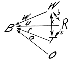
Three different approaches to causal inference had their origins in the 1920s. In a 1921 paper titled “Correlation and Causation,” published in the Journal of Agricultural Research, the American geneticist Sewall Wright introduced a method known as “path analysis.” In complex systems involving many uncontrollable and perhaps some unknown correlated factors — for instance when studying the weight and health of newborn animals — this method tries to measure the direct influence of each of the correlations and, as Wright explained, to find “the degree to which variation of a given effect is determined by each particular cause.” In order to do this, diagrams of variables connected by arrows are constructed, showing the various correlations within the system. (See Figure 1.) Based on these diagrams and the observed correlations between the variables, systems of equations can be constructed. The equations are then solved for the “path coefficients,” which represent the direct effects of variables on each other.
A generalization of path analysis known as “structural equation modeling” was subsequently developed. One application of this method is in studying mediation, in which a variable lies on the path between a cause and an effect. For example, stress can cause depression, but stress can also cause rumination, which can in turn cause depression. Rumination is thus a mediator of the causal effect of stress on depression. We might then wonder how much of the effect of stress on depression is mediated by rumination — that is, how much of the effect is on the indirect path between stress and depression (via rumination), compared to the direct path. The answer could help to determine whether interventions that target rumination might be more effective in reducing depression than interventions that target stress.
A second approach to causal inference had its origins in 1923, with a paper by the Polish statistician Jerzy Neyman introducing an early counterfactual account of causality in agricultural experiments. His methods were limited to experiments but were extended by Harvard statistician Donald Rubin in the 1970s to observational studies. Rubin’s causal model was based on the idea of “potential outcomes” — essentially counterfactuals.
An example will help illustrate again the problem with causation in observational studies we have been discussing. Consider patients who receive either treatment A or B, and are either cured or not. For each patient there is an outcome for treatment A and an outcome for treatment B, but only one of these outcomes is actually observed and the other one is merely potential. The causal effect for an individual patient is the difference between these two outcomes — cured or not cured depending on the treatment. But because it is not possible to observe both of the two potential outcomes — that is, a given patient cannot both receive a treatment and not receive it at the same time — the causal effect for an individual cannot be estimated. This is called the “fundamental problem of causal inference,” and on the face of it this would seem to be an insurmountable obstacle. However, while it is not possible to estimate an individual causal effect, it is possible — provided certain assumptions hold — to measure the average causal effect across a number of patients.
If the patients in question were enrolled in a randomized controlled trial that ran without a hitch (for example, no patients dropped out), then the necessary assumptions are easily satisfied. As discussed earlier, the outcomes of the patients in the two treatment groups can serve as substitute potential outcomes.
But suppose that the patients were not randomly assigned to treatment groups, and that this is instead an observational study. Unlike in an RCT, where patients in the two groups are likely to be very similar, in an observational study there may be substantial imbalances (in age, sex, wealth, etc.) between groups. There are a number of ways to address this problem using Rubin’s framework. Sometimes imbalances between groups can be dealt with using matching techniques that ensure the two groups are roughly similar. A related and more complex method is to estimate, for each patient, the probability that the patient would receive for example treatment A, given the patient’s characteristics. This estimate is known as a “propensity score,” first discussed in a 1983 paper that Rubin coauthored. Patients who received treatment B can then be matched with patients who received treatment A but who had similar propensity scores. This provides a general scheme for obtaining substitute counterfactuals that make causal inferences possible. An important caveat, however, is that this only works if all relevant variables — any of which could be confounders — are available. For example, the relationship between alcohol advertising and youth drinking behavior may be confounded by unmeasured factors such as family history and peer influence.
A third approach to causal inference, known as “instrumental variables analysis,” was introduced by economist Philip Wright (father of Sewall Wright) in his 1928 book The Tariff on Animal and Vegetable Oils. His method has been widely used in the field of econometrics, but more recently has been applied in other fields. In one application of it in a 1994 study, the effectiveness of treating heart attacks using aggressive medical techniques (catheterization and revascularization) was evaluated based on observational data from a group of Medicare beneficiaries. Those who were treated aggressively had much lower mortality rates than those who were not. It is easy to jump to the conclusion that aggressive treatment reduces mortality rates. However, as the study explained, the aggressively treated patients differed from the others in numerous ways — for instance, they were younger. And they may have also differed in ways that were not measured, such as the severity of their heart attacks. The risk is that — once the measured variables such as age are adjusted for, using a technique like matching — the unmeasured variables could still substantially bias results. Had the patients been randomized to receive different treatments, it would have been much easier to estimate the causal effect of aggressive treatment. But suppose a variable could be identified that was correlated with the type of treatment received (aggressive or not aggressive), did not directly affect the outcome, and was not likely to be correlated with any confounding variables. Such an “instrumental variable” can be used to form groups of patients such that patient characteristics are similar between groups, except that the likelihood of receiving the treatment in question varies between groups. In this way, an instrumental variable can be considered to be a sort of natural randomizer. In the heart attack study, patients who lived closer to hospitals that offered aggressive treatment were more likely to receive such treatment. The authors of the study realized that an instrumental variable could be based on a patient’s distance to such a hospital compared to the distance to their nearest hospital. This variable would not be expected to affect mortality except through the type of treatment received, nor would it be expected to affect other possible confounding variables. Provided these assumptions were valid, the instrumental variable approach could overcome unmeasured confounding to allow causal conclusions to be drawn. In this case, the instrumental variable analysis showed that aggressive treatment had the effect of lowering mortality only to a very small degree, in striking contrast to estimates using more conventional statistical methods. Far more important for lowering mortality, the study explained, was that patients received care within twenty-four hours of admission to the hospital.
Another application of the instrumental variable approach is to flawed randomized controlled trials. Consider an RCT of a drug in the form of a pill with an inactive pill (placebo) used as the control. If such a study is executed perfectly, it provides the best basis for drawing a conclusion about whether the drug affects patients’ outcomes. The trouble is that few RCTs are pulled off without a hitch. Common problems include patients dropping out or simply not taking all of their pills, which can introduce bias into the results. But even with these biases the random assignment to either the active pill or the placebo can be used as an instrumental variable that predicts the treatment actually received. Provided the necessary assumptions hold, an instrumental variable analysis can be used to give a valid estimate of the drug’s effect. Thus even in experimental settings, it may be necessary to apply methods of causal inference developed for observational studies.
As attractive as the instrumental variables approach is, it is not a panacea. Some of the key assumptions required cannot be tested, and serious biases can arise if they are violated. Notwithstanding its limitations, however, the instrumental variables approach can still be a powerful tool for causal inference.
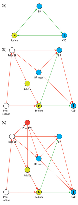
The late 1980s saw a resurgence of interest in refining methods of causal inference with the help of diagrams like those used in path analysis and structural equations modeling. These newer diagrams are known as “directed acyclic graphs” (DAGs) and have been widely used in computer science and epidemiology. The graphs are made up of nodes (commonly shown as circles) representing variables, connected by one-way arrows, such that no path leads from a node back to itself, which would represent a causal feedback loop (hence “acyclic”). (See Figure 2.) Powerful theorems about DAGs are available thanks to a branch of mathematics known as graph theory, used for modeling and analyzing relations within biological, physical, social, and information systems.
In order to specify a DAG for a particular problem, it is necessary to have some knowledge of the underlying causal structure. However, experts may disagree on the causal structure, and for a particular problem several different DAGs may be considered. Causal inferences obtained using this approach are always dependent on the particular assumptions encoded in a DAG. For example, when there is no arrow between two nodes, this indicates that there is no direct causal relationship between the variables represented by those nodes. Such an assumption can generate disagreement between experts, and may have a decisive effect on the analysis.
Before the era of DAGs, a number of different approaches for recognizing confounders were used. These have since been shown to be unreliable. For instance, some procedures for identifying confounders based on associations between variables may fail to identify certain confounders and wrongly identify others. This last point is critical because adjusting for the wrong variables could induce selection bias. A DAG encodes all the information necessary to determine which variables should be adjusted for, so as to remove confounders without inducing selection bias. However, except in the simplest cases, it is very difficult to determine by visual inspection of a DAG which variables should be adjusted for; using graph theory, algorithms have been developed that answer this question and others.
With the help of DAGs, the conditions that give rise to selection bias and confounding have been pinpointed, thereby settling an important question in the analysis of observational data.
Directed acyclic graphs have helped to solve other longstanding puzzles. Consider observational data on the relationship between a certain treatment and recovery from an illness. Suppose that patients who are treated are more likely to recover than those who are not. But when we examine the data on male and female patients separately, it turns out that among the males, those who are treated are less likely to recover; similarly, females who are treated are also less likely to recover. This reversal — known as Simpson’s paradox after the statistician Edward H. Simpson — may seem surprising, but it is a real phenomenon. This kind of situation can arise if the patients who receive treatment are disproportionately male, and the recovery rate for females is much lower than for males. Sex is thus a confounder of the relationship between treatment and recovery in this case, and the sex-specific results should be used for decision-making about the treatment’s effectiveness: the treatment is not helpful.
But Simpson’s paradox has another surprising aspect. Suppose that the treatment is suspected of having an effect on blood pressure, and instead of breaking the data down by sex, the breakdown is by high versus low blood pressure one week into treatment (or at roughly the same time in the untreated group). Imagine that the data of the two groups — high and low blood pressure — are like the data of the two groups broken down by sex in the earlier scenario. As before, the patients who are treated are more likely to recover than those who are not, yet within both of the subgroups (high and low blood pressure) the patients who are treated are less likely to recover. But in this case blood pressure, unlike sex, is not a confounder of the relationship between treatment and recovery, since it is not a common cause of treatment and recovery. In this scenario, the overall results rather than the subdivided results should be used for decision-making.
The paradox that today carries Simpson’s name was first identified at the beginning of the twentieth century, but Simpson examined it in detail in a 1951 paper and noted that the “sensible” interpretation of the data should sometimes be based on the overall results and sometimes on the subdivided data. However, Simpson’s analysis left unclear what the general conditions are for when to use the overall results and when the subdivided data. All he could show was that considering the context of the data was essential for interpreting it. No statistical method or model was available for solving the problem. In a 2014 paper published in The American Statistician, one of the most notable researchers in this field, Israeli-American computer scientist Judea Pearl, has provided an answer to this longstanding question. He showed that in situations where there is a Simpson’s-paradox-style reversal, if a DAG can be specified, causal graph methods can determine when to use the overall results and when to use the subdivided data.
Reflecting on Simpson’s contribution, Pearl notes that Simpson’s thinking was unconventional for his time: “The idea that statistical data, however large, is insufficient for determining what is ‘sensible,’ and that it must be supplemented with extra-statistical knowledge to make sense was considered heresy in the 1950s.” Causal questions cannot be answered simply by applying statistical methods to data. In particular, subject-matter knowledge is critical. And with the development of DAGs and other tools we now have formal procedures to bring subject-matter knowledge to bear on these problems.
As applications of causal inference are becoming increasingly common in a variety of fields — not only in computer science and medicine but also in sociology, economics, public health, and political science — it is appropriate to consider the achievements and limitations in this field over the course of the near-century since Sewall Wright’s groundbreaking contributions to causal inference, his path analysis. The advances since the 1920s have truly been transformative, with the development of ever more sophisticated methods for solving complex problems, especially in fields such as epidemiology that rely largely on observational data rather than experiments. Much progress has been made in untangling the difficulties surrounding counterfactuals — of finding ways to know what would have happened if a given intervention, such as a medical treatment, had not occurred. Tools like the randomized controlled trial have become so widely accepted that it is hard to imagine our world without them.
Meanwhile, questions of causation — what it is, how it differs from correlation, how our best statistical methods try to answer these questions — remain obscure to most, especially as news reports often play fast and loose with cause and effect. And while there has been significant progress toward integrating the major approaches to causal inference, no grand unified theory has arisen. Philosophers, too, continue to wrestle with causation, both at a foundational level — for instance debating theories of causation and sorting out the difference between causally related and causally unrelated processes — and in particular areas, such as the question of free will and whether our thoughts and actions are neurochemically caused or freely chosen. Psychologists study the question of causal attribution — how, as individuals, we identify and explain the causes of events and behavior. Historians strive to ascertain the causes of historical events. And in our personal lives as well as in the law we often struggle with questions of causation and personal and legal responsibility.
One of the greatest challenges is the intricacy of the causal relationships that underlie so many phenomena: What causes today’s weather? What are the effects of violent video games? What will be the results of a tax increase? Causal diagrams have made a substantial contribution to our ability to analyze such complex situations — but they can yield unreliable conclusions if the causal structure is incorrectly specified.
Hume’s point stands: correlation can be directly observed, but never the causal link between one event and another. Causal inference depends on more than just the data at hand; the validity of the conclusions always hinges on assumptions — whether they are based on external evidence, expert background knowledge, theory, or guesswork. Curiously, the current excitement about big data has encouraged in some people the opposite notion. As Chris Anderson writes:
Petabytes allow us to say: “Correlation is enough.” We can stop looking for models. We can analyze the data without hypotheses about what it might show. We can throw the numbers into the biggest computing clusters the world has ever seen and let statistical algorithms find patterns where science cannot.
Such grandiose visions suggest a failure to understand the limits of brute-force computation. While it is possible to detect useful correlations by applying sheer computing power to massive databases, by themselves correlations cannot answer questions about the effectiveness of interventions nor can they explain underlying causal mechanisms, knowledge of which is often critical for making decisions, most obviously perhaps in medicine where our health and our lives are at stake. To address such issues we need to judiciously consider causation, and that is not a matter of brute force.
Exhausted by science and tech debates that go nowhere?